Doing linear regression in Excel is simple. Now I’d like to show you how exactly this is done.
Let’s use the same data set:
| x | 9.42 | 2.78 | 5.87 | 5.49 | 6.48 | 4.91 | 7.82 | 2.70 | 2.65 | 8.42 | 5.85 | 0.93 |
| y | 52.24 | 4.15 | 13.72 | 7.00 | 5.28 | 6.98 | 42.00 | 7.15 | 3.41 | 31.00 | 12.59 | 1.09 |
Let’s say we want do a order-2 linear regression. That means, we want a function:
f(x)=c*x^2 + b*x+a
a, b and c should be chosen in a way such that if we put x into f(x), the difference/error between f(x) and y, will be minimized, in the least square sense.
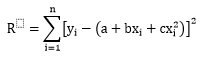
So we have the difference R as a function of a,b,c:
R(a,b,c)=(c* 9.42^2 + b* 9.42 + a – 52.24)^2+(c*2.78^2+b*2.78+a-4.15)^2+…+(c*0.93^2+b*0.93+a)
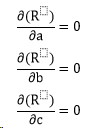
R is smooth every where in space. So R is minimal where:
D(R)/D(a)=0; D(R)/D(b)=0; D(R)/D(c)=0
Now we’ll have to employ the compact form to avoid tedious typing:
In order for R to be minimal, we need:
Insert R into the equations and expand them, we get:
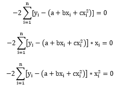
That is:
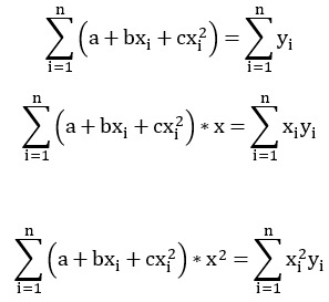
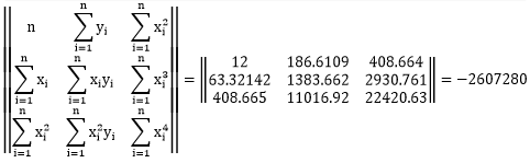
Or in matrix form:
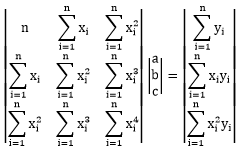
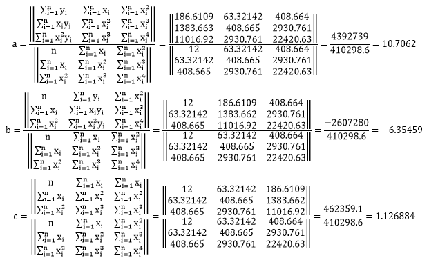
Now this is a very simple equation, so we can simply solve it using Cramer’s rule:
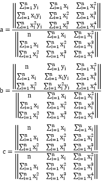
It looks scary but actually not too complex. We need the sum of x, x^2, x^3, x^4, x*y and x^y. We can actually verify this in excel:
| x | y | x^2 | x^3 | x^4 | x*y | x^2*y |
| 9.42 | 52.24 | 88.69578 | 835.323 | 7866.942 | 491.974 | 4633.334 |
| 2.78 | 4.15 | 7.721688 | 21.45697 | 59.62447 | 11.53932 | 32.06537 |
| 5.87 | 13.72 | 34.43254 | 202.0476 | 1185.6 | 80.52797 | 472.5321 |
| 5.49 | 7.00 | 30.18894 | 165.8715 | 911.3719 | 38.47401 | 211.3934 |
| 6.48 | 5.28 | 41.99053 | 272.099 | 1763.204 | 34.19838 | 221.6059 |
| 4.91 | 6.98 | 24.08858 | 118.227 | 580.2595 | 34.23907 | 168.0457 |
| 7.82 | 42.00 | 61.22442 | 479.0568 | 3748.43 | 328.6334 | 2571.426 |
| 2.70 | 7.15 | 7.269068 | 19.59829 | 52.83935 | 19.27266 | 51.96143 |
| 2.65 | 3.41 | 7.003793 | 18.53532 | 49.05312 | 9.028243 | 23.89296 |
| 8.42 | 31.00 | 70.90802 | 597.0945 | 5027.948 | 261.0414 | 2198.149 |
| 5.85 | 12.59 | 34.27254 | 200.6409 | 1174.607 | 73.71933 | 431.5732 |
| 0.93 | 1.09 | 0.869064 | 0.810173 | 0.755272 | 1.014426 | 0.945685 |
| 63.32 | 186.61 | 408.665 | 2930.761 | 22420.63 | 1383.662 | 11016.92 |
So we have:
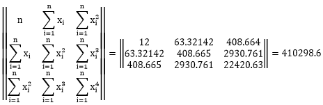
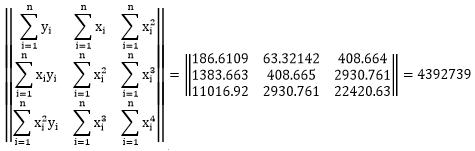

So in the end we get:
This is exactly what Excel displayed on the chart:
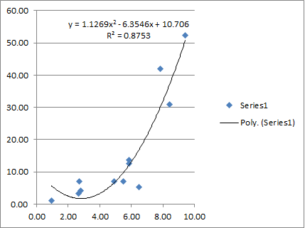
I actually put all this in an Excel file so you can try it yourself. Please note that in the excel file we have a data set of 12 points. If your data set has a different size, you may have to adapt the formulas a little bit. 🙂