Linear regression in Excel

Excel has a very handy feature that does linear regression for you very intuitively.

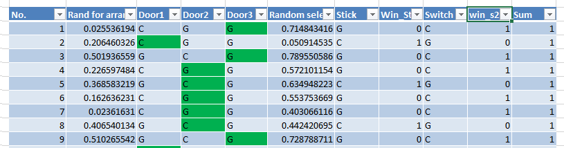
Let’s say you have a data set like this:

x 9.42 2.78 5.87 5.49 6.48 4.91 7.82 2.70 2.65 8.42 5.85 0.93
y 52.24 4.15 13.72 7.00 5.28 6.98 42.00 7.15 3.41 31.00 12.59 1.09

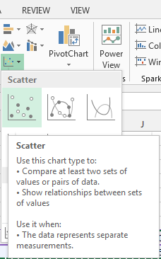
First, you’ll have to insert a scatter chart:

insert_scatter_chart

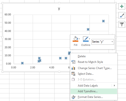
You’ll get a chart like this (Excel is smart enough to figure out what should be the x-axis and what should be the y-axis):

scatter_chart_ex1

Now, right click on the dots and then you can select “Add Trendline…” from the pop-up menu.

add_trendline

Then you’ll be presented with a dialog like this:

trend_line_options

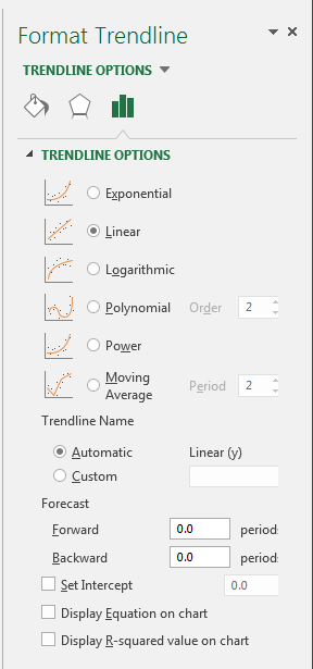
Note that Excel has different options for “Linear” and “Polynomial”. Here the option is about the relationship between the variables. All these different options are all Linear Regressions.

Let’s try a order 2 polynomial regression and check the option “Display Equation on chart” and “Display R-squared value on chart”. This is what you’ll get:

order_2_regression

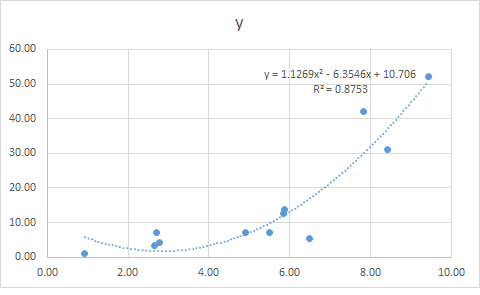
Good thing about doing this in Excel is, you can always change the data set and your chart and equation will be updated automatically.

Depending on the nature of your data set, you may want to try different model to get a better fit, the procedure will be the same.

Monty Hall Problem simulation in Excel

Monty Hall Problem is definitively the most confusing puzzle among educated people. After explaining this to different colleagues and friends (With a success rate below 50%), I found it’s easier simply presenting the fact. So here’s a simulation of it in excel.

monty_hall_excel

Let’s me explain a little bit about this excel:

Each row in the table is a test case, or an experiment.

In each such a experiment, a random number is generated to determine where do we put the car. A goat will be placed behind each of the rest doors. So in the table, we have “C” denotes a Car and “G” denotes a goat.

If the number is between 0-1/3, then the car will be placed behind Door1. If the number is between 1/3-2/3, then the car will be placed behind Door2. If the number is between 2/3-1, then the car will be placed behind Door3.

Then in the 6th column of the table, another random number is generated to determine the 1st choice.

Again, if the number is between 0-1/3, that means the guest chose Door1 in the first attempt. If the number is between 1/3-2/3, then the guest chose Door2 in his/her first attempt. If the number is between 2/3-1, then he/she chose Door3 in his/her first attempt.

Note that both of the 2 random numbers have a unify distribution between 0 and 1. And the 2 numbers are completely independent to each other.

Also in the table, the guest’s first choice is high-lighted in green.

The next column, the 7th column, shows what the guest will get if he sticks to his/her first attempt. And the 8th column shows whether he/she wins a car or not. (1 wins, 0 loss).

The 9th column shows what the guest will get if he/she switches to the other door when he/she is given another chance. And the next column shows whether he/she will win or not if he switches.

In the end of the table, after 400+ experiments, the outcome of the 2 strategy was summed up. Out of 432 experiments, you’ll get a car 142 times, if you stick to your original choice, you’ll get a car 290 times, if you switch.

The good thing about this excel is, you can simply press F9 and ask Excel to recalculated and see with your own eyes of the outcome.