以下内容是我从牛津大学Jon Chapman的讲座中总结记录的。
Chapman研究了Escher的画,Print Gallery。

他有如下发现:
- 在图像中旋转一周,则似乎画面中所有的东西都在放大,但是放大一圈之后,又跟原来一样了。

这种特性让Chapman想到了Droste Effect,其特点就是缩放不变。
以下内容是我从牛津大学Jon Chapman的讲座中总结记录的。
Chapman研究了Escher的画,Print Gallery。
他有如下发现:
这种特性让Chapman想到了Droste Effect,其特点就是缩放不变。
My copy of Escher’s artwork got some attention and quite some people asked me, “what kind of programmer are you?”, well, this Youtube video explains it well.
Actually, Joma’s video basically depicted me when in real dev mode. Upon watching this video, I couldn’t wait to re-implement it in Python. However, the initial version is basically a trans-coding of the original C code and was pretty hard to read. So here is a version that actually uses Matrix multiplication in Python (In the mean time, I still have to fix the syntax highlighter…):
import timeimport numpy as npscreen_size = 40theta_spacing = 0.07phi_spacing = 0.02illumination = np.fromiter(".,-~:;=!*#$@", dtype="<U1")A = 1B = 1R1 = 1R2 = 2K2 = 5K1 = screen_size * K2 * 3 / (8 * (R1 + R2))def render_frame(A: float, B: float) -> np.ndarray:"""Returns a frame of the spinning 3D donut.Based on the pseudocode from: https://www.a1k0n.net/2011/07/20/donut-math.html"""cos_A = np.cos(A)sin_A = np.sin(A)cos_B = np.cos(B)sin_B = np.sin(B)output = np.full((screen_size, screen_size), " ") # (40, 40)zbuffer = np.zeros((screen_size, screen_size)) # (40, 40)cos_phi = np.cos(phi := np.arange(0, 2 * np.pi, phi_spacing)) # (315,)sin_phi = np.sin(phi) # (315,)cos_theta = np.cos(theta := np.arange(0, 2 * np.pi, theta_spacing)) # (90,)sin_theta = np.sin(theta) # (90,)circle_x = R2 + R1 * cos_theta # (90,)circle_y = R1 * sin_theta # (90,)x = (np.outer(cos_B * cos_phi + sin_A * sin_B * sin_phi, circle_x) - circle_y * cos_A * sin_B).T # (90, 315)y = (np.outer(sin_B * cos_phi - sin_A * cos_B * sin_phi, circle_x) + circle_y * cos_A * cos_B).T # (90, 315)z = ((K2 + cos_A * np.outer(sin_phi, circle_x)) + circle_y * sin_A).T # (90, 315)ooz = np.reciprocal(z) # Calculates 1/zxp = (screen_size / 2 + K1 * ooz * x).astype(int) # (90, 315)yp = (screen_size / 2 - K1 * ooz * y).astype(int) # (90, 315)L1 = (((np.outer(cos_phi, cos_theta) * sin_B) - cos_A * np.outer(sin_phi, cos_theta)) - sin_A * sin_theta) # (315, 90)L2 = cos_B * (cos_A * sin_theta - np.outer(sin_phi, cos_theta * sin_A)) # (315, 90)L = np.around(((L1 + L2) * 8)).astype(int).T # (90, 315)mask_L = L >= 0 # (90, 315)chars = illumination[L] # (90, 315)for i in range(90):mask = mask_L[i] & (ooz[i] > zbuffer[xp[i], yp[i]]) # (315,)zbuffer[xp[i], yp[i]] = np.where(mask, ooz[i], zbuffer[xp[i], yp[i]])output[xp[i], yp[i]] = np.where(mask, chars[i], output[xp[i], yp[i]])return outputdef pprint(array: np.ndarray) -> None:"""Pretty print the frame."""print(*[" ".join(row) for row in array], sep="\n")if __name__ == "__main__":for _ in range(screen_size * screen_size):A += theta_spacingB += phi_spacing# clear screen using ANSI control codeprint("\x1b[H")time.sleep(0.05)pprint(render_frame(A, B))
听说Escher,是在大学时候看到这本书:

这是Gödel, Escher, Bach: an Eternal Golden Braid一书的中文简译,本来就比较抽象艰深,再进行翻译和简化转述,文字看得半懂不懂,图片倒的确是看的津津有味。


右图就是我们要山寨的Print Gallery:
The notion of 1+2+3+4+…=-1/12 has become so wide spread that quite a few of my friends actually feel convinced that it’s actually a true statement in general, even though it is very counter intuitive.
The point is, in order to evaluate an expression, that expression has to be well-defined.
Expressions like a+b is well defined in the sense that we know it is a binary operation, we know what are we supposed to do to get the result.
Expressions like a+b+c+… is not well defined, because there are multiple operators involved, and the order of evaluation is not clearly specified.
Take the sum of the alternating series as an example:
摩西快速学习了算术和几何……
这些知识他是从埃及人那里学到的。埃及人研习数学和其它学问。《形而上学》亚里士多德
算法 是用以完成某项计算任务的有限步骤。算法跟计算机编程有紧密的联系,以至于大多数知道这个词的人以为算法的使用是从计算机科学开始。但实际上,人们使用算法已经有几千年的历史。数学中充满了算法,有一些我们到今天还在使用。学生们学习的长加法就是一种算法。
尽管使用算法的历史很长,算法这个概念并不是一开始就存在,它是后来发明出来的。尽管我们不知道是谁首先发明了这个概念,却明确知道有些算法至迟在4000多年前的古埃及就存在了。
古埃及文明的核心是尼罗河,因为其农业有赖于尼罗河泛滥带来的肥沃泥土。问题是,尼罗河一发水,用来划分权属的界标也都被冲掉了。埃及人惯用绳子测量长度,因此发展出一套方法,可以根据书面记录重建界标。一群制定的祭司专司此事,他们学过这些数学技术,因此成为“拉绳子的人(rope-strecher)”。希腊人后来会把他们叫做几何学家(geometers),意思是“土地丈量者”。
很不幸我们并没有多少古埃及数学知识的文字记录,当时的数学文件仅有两篇留存至今。我们关心的一个,叫做Rhind Mathematical Papyrus,名字来自于19世纪在埃及买到它的苏格兰收藏者。这篇文献成于约公元前1650年,抄写者名叫Ahmes。文献中有一系列算术和几何问题,还有一些辅助计算的表格。其中包含一个快速乘法技术和一个快速除法技术,是最早的有记录的算法。我们首先来看一看这个快速乘法算法,(我们很快会看到)它至今仍然是重要的计算技术。
跟其它古文明一样,埃及人使用的数字系统中没有数位概念,也没有零。因此,乘法非常复杂,只有少数专家能够掌握。(想象一下只使用罗马数字进行两位数乘法)
首先,什么是乘法?粗略地说,乘法就是“把一个数跟它自身反复相加”。严格一些,我们可以首先把乘法分为两种情况:乘以1,或者乘以一个大于1的数。
乘数为1的乘法的定义是:
$$1a=a$$ (2.1)
然后,我们考虑如何计算比我们已经计算出来的再多一倍的情形。有些读者可以意识到这是一个递推,我们会在后面正式使用这个技术。
$$(n+1)a=na+a$$ (2.2)
计算na的厂家做法是把n个a加起来。但是,在n很大的时候,这可能非常繁琐,因为需要进行n-1次加法。使用C++,这个算法是这样的:
int multiply0(int n, int a){
    if (n==1) return a;
    return multiply0(n-1, a)+a;
}
这样两行代码对应于(2.1)和(2.2)。a和n都必须是正数,古埃及当时的约定也是如此。
Ahmes所描述的算法,这个算法在古希腊被称为“埃及乘法”,而很多现代作者则称之为“俄罗斯农民算法”,建立在如下洞察上:
$$ 4a=((a+a)+a)+a=(a+a)+(a+a) $$
这个优化利用了加法的结合律:
$$a+(b+c)=(a+b)+c $$
这样,我们只需要计算一次a+a,减少了计算次数。
核心思想在于,不断地把n取半,同时把a加倍,使用数的2的次方倍相加来计算乘法结果。在当时,人们不会使用变量a和n来描述算法,而是由作者给出示例,然后说“其它数字同理”。Ahmes也是这么做的,他使用下面的表格来演示这种算法,n=41,a=59:
1 ♦ 59
2 118
4 236
8 ♦ 472
16 944
32 ♦ 1888
每个条目的最左边是2的幂,右边是前一条目的数字的倍数(数字加倍相对容易计算)。有标记的值对应41的二进制表示中数值为1的位。这个表格的意思是说:
$$41*59=(1*59)+(8*59)+(32*59)$$
其中右边的每一个乘积可以由对59加倍响应的次数而得到。
这个算法需要检查n是奇数还是偶数,所以我们可以推断古埃及人知道它们的区别,尽管我们没有直接的证据,但是古希腊人,他们自称从古埃及人那里学到数学,显然知道奇偶的区别。下面是他们的定义方法用现代数学标记表达出来:
$$n=n/2+n/2$$ 说明n是偶数
$$n=(n-1)/2+(n-1)/2+1$$ 说明n是奇数
我们也将使用这个特点:
odd(n) 意味着 half(n)=half(n-1)
下面是埃及乘法的C++实现:
int multiply1(int n, int a){
    if (n==1) return a;
    int result=multiply1(half(n), a+a);
    if (odd(n)) result=result +a;
    return result;
}
odd(x)很容易实现,测试x的最低位就可以了,half(x)则可以通过对x进行一次右移实现:
bool odd(int n) { return n&0x1;}
int half(int n) { return n>>1; }
multiply1需要进行多少次加法运算?每次调用这个函数,我们需要在a+a的地方进行一次加法,因为我们是不断对n取半,我们需要调用这个函数logn次。在某些时候,我们还需要在result+a的地方进行加法运算,因此加法运算的总次数为:
$$\#(n)=logn + v(n)-1$$
其中v(n)是n的二进制表达中1的个数(population count或者pop count)。由此我们把一个O(n)算法优化成了O(logn)算法。
这个算法已经最优了吗?不见得。比如,如果我们要乘以15,使用之前的公式,我们需要
$$\#(15)=3+4-1=6$$
进行6次加法。但是我们使用下面的办法,就只需要5次加法运算:
int multiply_by_15(int a){
    int b=(a+a)+a;    //b == 3*a
    int c+b+b;        //c == 6*a
    return (c+c)+b;   //12*a + 3*a
}
这样一系列加法运算又称为加法链。这里我们发现了15的最优加法链,尽管如此,Ahmes的算法在多数情况下已经足够好了。
为n<100的数找到最优加法链
有读者可能已经注意到其中有些乘法运算可以更快,只要我们在第一个参数大于第二个参数的情况下交换一下参数顺序就可以了(比如,3*15会比15*3更容易计算)。的确如此,而且古埃及人也知道这一点。但是我们不会在这里进行这样的优化,因为到第七章我们会发现,我们最终要把算法推广到不同的数据类型。在这种情况下,参数的顺序是不能交换的。
函数multiply1的加法运算次数还可以,但是它还要进行logn次递归调用。鉴于函数调用的开销很高,我们希望能够优化程序以避免这个开销。
我们将要利用的一个原则是:It is often easier to do more work rather than less. 特别地,我们准备计算
r+na
其中r是加法计算的中间结果,也就是说,我们要实现一个乘法累计函数,而不仅仅是乘法函数。这种思维方式不仅仅适用于程序编写,也适用于硬件设计和数学——比如在数学中,时常有一般性判断比特定判断更容易证明的情形。
这里是我们的乘法累计函数:
int mult_acc0{int r, int n, int a) {
    if (n==1) return r+a;
    if (odd(n)){
        return mult_acc0(r+a, half(n), a+a);
    }else{
        return mult_acc0(r, half(n), a+a);
    }
}
这里有一个不变形式:r+na=r0+n0a0,其中r0、n0和a0是r、n和a这些变量的初始值。
我们可以通过简化递归获得进一步优化。注意在上面的两行递归调用代码只有第一个参数不同,这样对于奇数情况和偶数情况分别进行递归,不如我们在进行递归前根据情况修改第一个参数的值:
int mult_acc1(int r, int n, int a) {
    if (n==1) return r+a;
    if (odd(n)) r=r+a;
    return mult_acc1(r, half(n), a+a);
}
现在我们的函数是尾递归函数——递归仅仅发生在返回值里面——我们马上会利用这一特点。
我们注意到两点:
因此,我们可以首先判断n的奇偶性,这样把n与1进行比较的次数降低一半:
int mult_acc2(int r, int n, int a) {
    if (odd(n)) {
        r=r+a;
        if (n==1) return r;
    }
    return mult_acc2(r, half(n), a+a);
}
有些程序员认为编译器可以为我们做这样的优化,其实不太可能。编译器不能把一种算法优化成另外一种算法。
到目前为止都很好,不过我们的目标是避免递归以节省函数调用的开销。要达到目的,如果我们的函数是完全尾递归就好了。
定义2.1 一个完全尾递归函数是一个所有递归调用的形式参数都跟函数本身一致的函数。
同样地,我们可以通过在递归调用之前给变量重新赋值来达到这个要求:
int mult_acc3 (int r, int n, int a) {
    if (odd(n)) {
        r=r+a;
        if (n==1) return r;
    }
    n=half(n);
    a=a+a;
    return mult_acc3(r,n,a);
}
到了这里,把它转化成一个循环就很简单了,只需要使用一个while(true)结构替换掉尾递归就可以了:
int mult_acc4(int r, int n, int a) {
    while (true) {
        if (odd(n)) {
            r=r+a;
            if (n==1) return r;
        }
        n=half(n);
        a=a+a;
    }
}
使用这个全新的乘法累加函数,我们可以写一个新版的乘法函数:
int multiply2(int n, int a) {
    if (n==1) return a;
    return mult_acc4(a, n-1, a);
}
注意我们在调用mul_acc4的时候预先把累加结果置为a,这样就减少了一次循环。
效果很不错,除了在n是2的幂的时候。由于我们第一次调用就把n减去1,这样mult_acc4函数被调用的时候第二个参数是一个二进制表达是全1的数,这对于我们的算法是最坏情况。因此,我们要在n是偶数的情况下做一些预处理,以避免这种情形。我们把n取半(同时把n加倍),直到n变成奇数。
int multiply3(int n, int a) {
    while (!odd(n)) {
        a=a+a;
        n=half(n);
    }
    if (n==1) return a;
    return mult_acc4(a, n-1, a);
}
但这样的话,mul_acc4就没有必要再检查n=1的情况了,因为n是奇数,n-1是偶数。因此,我们可以在调用的时候直接把n-1取半,把a再加倍,这样就是我们的最终版:
int multiply4(int n, int a) {
    while (!odd(n)) {
        a=a+a;
        n=half(n);
    }
    if (n==1) return n;
    return mult_acc4(a, half(n-1), a+a);
}
在不断变换我们的乘法算法的过程中,可以看到重写代码是很重要的。没有谁一上来就能写出很好的代码,很多时候需要反复尝试才能找到最高效或者最通用的方法。程序员不应该有一遍就过的想法。
在重写过程中你可能会想,一条指令的多少不见得能造成多大的区别。但是也可能你的代码在后来很长时间内被重用很多次(实际上,临时处理措施经常变成代码里面存活时间最长的部分),而且,本来可以省掉的操作现在不起眼,留下来也可能会被修改成非常开销非常高的代码。
努力追求效率的另外一个好处是,在此过程中你不得不逼迫自己深入理解问题本身。与此同时,理解深入必然带来更有效率的实现,这是一个良性循环。
初等代数的学生都会学习如何通过变换表达式的形式来简化它们。在我们实现埃及乘法的不同实现中,我们也经历了类似的变换过程,重新安排代码语句,使之更清晰更高效。每个程序员都应该养成尝试对代码进行变换的习惯,直到得到最佳形式。
本章我们看到了数学在古埃及是怎样出现的,如何留下了第一个有记录的算法。我们要到靠后面的内容才会回到这个算法并对其进行推广。接下来,我们要向后跳跃1000年,领略一些古希腊人的数学发现。
中文版见这里。
This is inspired by a post on Quora by Alon Amit. I found this approach of defining e, the Euler number more intuitive than the traditional way($$e=\lim_{n \to \infty} (1+\frac{1}{n})^n$$). In addition, it explains the importance of the Euler number very well.
First of all, we need a function that solves the elementary differential equation:
$$\frac{d f(x)}{d x} = f(x)$$
Of course, without specifying an initial value, this equation will have infinite number of solutions. Just for convenience, let’s specify:
$$f(0)=1$$
By Picard–Lindelöf theorem, our equation:
$$\begin{gather*} \frac{d f(x)}{d x} = f(x)\\f(0)=1 \end{gather*} $$
has one and only one solution.
Now, let’s see what kind of property this function $$f(x)$$ has.
在传统教科书里,欧拉数$$e$$通常被定义为:
$$e=\lim_{n \to \infty} (1+\frac{1}{n})^n$$
然后在后续的讨论中发现$$e$$的种种奇妙性质。前一段在Quora上看到Alon Amit解释了$$e$$的来源,觉得这种新的定义方式一方面更直观,另一方面从一开始就展示了$$e$$为什么很重要。
首先,如果我们把微分运算看成一种函数映射,那么在该映射下保持形式不变的函数就非常重要了。这个函数满足:
$$f’=f$$ ……(1)
如果我们加上初值条件$$f(0)=1$$,根据存在性和唯一性定理,该微分方程有且只有一个解。
要解这个方程,我们有如下观察:
首先,忽略初始条件,如果$$f(x)$$是一个解,则$$c*f(x)$$也是解。其中$$c$$为任意常数。因此$$c*f(x)$$就是方程$$f’=f$$的解空间。
其次,注意到,如果$$f(x)$$是一个解,则$$f(x+a)$$,其中$$a$$为任意常数也是一个解。根据前面的讨论,我们得到:
$$f(x+a)=c*f(x)$$ ……(2)
也就是说,对函数曲线在水平方向进行平移,等同于对函数曲线在垂直方向上进行缩放。
此时我们把初值条件$$f(0)=1$$代入(2),得到$$f(a)=c$$。再带回(2),得到:
$$f(x+a)=f(a)*f(x)$$
由此我们知道,符合方程(1)的解,一定是一个指数函数。唯一的问题是,这个指数函数的底是多少。
刚好,很容易验证函数$$exp(x)=1+x+\frac{x^2}{2!}+\frac{x^3}{3!}+…+\frac{x^n}{n!}+…$$是方程(1)的解。因此,
$$f(1)=exp(1)=1+1+\frac{1}{2!}+\frac{1}{3!}+…+\frac{1}{n!}+…$$
不难证明,该级数是收敛的,而它就是我们要找的指数函数的底。
简单地说,$$e$$是基本微分方程
$$\begin{gather*} \frac{d f(x)}{d x} = f(x)\\f(0)=1 \end{gather*} $$
的解。而这个基本微分方程在动力学、电磁学、通信以及概率论中都有非常基础的地位,因此,$$e$$才特别重要。
比如,在电学中非常基础的LC电路,其微分方程样式实际上是:
$$\frac{d^2I}{dt^2}=-cI$$,其中$$c$$为大于零的常数。
令$$I(t)=e^{k*t}$$,其中$$k$$为常数,代入方程得到:
$$k^2*e^{k*t}=-c*e^{k*t}$$,因此,
$$k^2=-c\\k=\pm\sqrt{c}*i$$
其中,$$i=\sqrt{-1}$$。因此,$$I(t)$$的通解为$$e^{\sqrt{c}*i}$$和$$e^{-\sqrt{c}*i}$$的线性组合。
相应的方程形式还出现在弹簧模型,电磁波方程以及正态分布中。是因为有了$$exp(x)=e^x$$这个基础,我们才能够解这些方程。这就是为什么$$exp(x)=e^x$$这么重要,为什么$$e$$这么重要。
相对而言,把$$e$$定义为$$\lim_{n \to \infty} (1+\frac{1}{n})^n$$,然后推导相应的性质,不如这样定义$$e$$来的直观。
英文版见这里。
注,后续搜索发现,认为$$e$$的重要性来自于$$e^x$$的导数就是其自身的看法很有渊源。英文维基的exponential function页面说,
The reason this number e is considered the “natural” base of exponential functions is that this function is its own derivative.
其来源之一是R柯朗的数学是什么,其中说到:
This natural exponential function is identical with its derivative. This is really the source of all the properties of the exponential function, and the basic reason for its importance in applications…
可见自己当年看书还是不细致。。。
中学以来,我粗浅的音乐知识一直告诉我,不同的音高其实就是不同的频率。具体地说,乐音的基频决定了它的音高,泛音的组合关系决定了它的音色。
但是,实际情况可能要复杂的多。在尝试用Matlab作曲时我发现,用频率组合的思路,很难产生真实的乐器发出的声音。这也是为什么第二部分一直难产,我没拿准频率组合的思路最终可以做到什么程度。
这几天在看维基的时候才发现,根本的问题在于,音高并不等同于频率。频率是一个可测量的物理指标,而音高是人类大脑对于频率组合的总体解读。这个解读跟乐音的基频有很大关系,但是不绝对。
这么说可能很抽象,还是简单看一个例子(来自维基百科):
这一段音乐的独特之处在于,听上去,音高在1分钟时间内一直在降低,而实际上音乐是重复的(都不用分析频率)。
频谱图在这里,这里的频率是线性坐标:

更多的信息请查看:
I have been attempted to do this for a long time, but only now I have some time to actually try it out. As it turned out, to have Matlab playing music is relatively easy, to have Matlab playing appealing music is way harder than I have imagined.
The core part is this Matlab function:
sound(v);
This function takes a vector and simply output it to the audio device in sequence. Values in the vector is the relative amplitude. Values larger than 1 will be ignored.
The default sample rate is 8000, so you’ll need 8000 data point to get 1 second of sound. If we want higher sample rate, then have to play the vector at a higher sample rate:
sound(v,16000);
Now, it’s very easy to generate such a vector:
First, generate a vector that represents time points:
tp=0:1/16000:0.5;
v=sin(440*2*pi*tp);
The first line generates a vector of 0.5*16000 values. That is 0.5 seconds in 16000 sample rate. The second line generates a sine wave of 440Hz for 0.5 seconds.
440Hz is A4. 12 half tones double the frequency. From C4 to A4 is 9 half tones. So C4 is 440*2^(-9/12)Hz. So for a simple C4 to C5, here’s the frequencies:
σ=2^(1/12)
| Note | Numbered Notation | Frequency |
| C | 1 | 440*σ^-9 |
| C# | 440*σ^-8 | |
| D | 2 | 440*σ^-7 |
| D# | 440*σ^-6 | |
| E | 3 | 440*σ^-5 |
| F | 4 | 440*σ^-4 |
| F# | 440*σ^-3 | |
| B | 5 | 440*σ^-2 |
| B# | 440*σ^-1 | |
| A | 6 | 440 |
| A# | 440*σ | |
| G | 7 | 440*σ^2 |
| C | i | 440*σ^3 |
So we can simply do this:
n1=sin(440*2^(-9/12)*2*pi*tp);         % C
n2=sin(440*2^(-9/12)*2*pi*tp);         % C
n3=sin(440*2^(-2/12)*2*pi*tp);         % B
n4=sin(440*2^(-2/12)*2*pi*tp);         % B
n5=sin(440*2^(0/12)*2*pi*tp);          % A
n6=sin(440*2^(0/12)*2*pi*tp);          % A
n7=sin(440*2^(-2/12)*2*pi*tp);         % B
sound(n1,16000);
sound(n2,16000);
sound(n3,16000);
sound(n4,16000);
sound(n5,16000);
sound(n6,16000);
sound(n7,16000);
This gives us “twinkle twinkle little star”. Here I output the audio into .wav file:
wavwrite([n1,n2,n3,n4,n5,n6,n7],16000,'c:\twinkle.wav');
Easy, right?
On hearing it, you notice that, it sounds very uncomfortable, and there’s no variation of amplitude within one note.
The problem is, I’m using “pure tone” here. Real instruments generate sound with a very rich composition of different frequency, phase and amplitude, that we haven’t take into consideration here. Next post I’ll try to mimic the sound generated by a hitting a key on a piano.
Doing linear regression in Excel is simple. Now I’d like to show you how exactly this is done.
Let’s use the same data set:
| x | 9.42 | 2.78 | 5.87 | 5.49 | 6.48 | 4.91 | 7.82 | 2.70 | 2.65 | 8.42 | 5.85 | 0.93 |
| y | 52.24 | 4.15 | 13.72 | 7.00 | 5.28 | 6.98 | 42.00 | 7.15 | 3.41 | 31.00 | 12.59 | 1.09 |
Let’s say we want do a order-2 linear regression. That means, we want a function:
f(x)=c*x^2 + b*x+a
a, b and c should be chosen in a way such that if we put x into f(x), the difference/error between f(x) and y, will be minimized, in the least square sense.
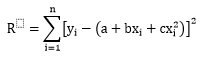
So we have the difference R as a function of a,b,c:
R(a,b,c)=(c* 9.42^2 + b* 9.42 + a – 52.24)^2+(c*2.78^2+b*2.78+a-4.15)^2+…+(c*0.93^2+b*0.93+a)
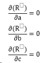
R is smooth every where in space. So R is minimal where:
D(R)/D(a)=0; D(R)/D(b)=0; D(R)/D(c)=0
Now we’ll have to employ the compact form to avoid tedious typing:
In order for R to be minimal, we need:
Insert R into the equations and expand them, we get:
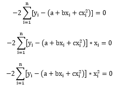
That is:
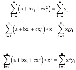
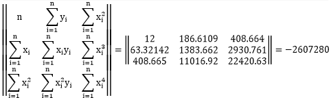
Or in matrix form:
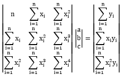
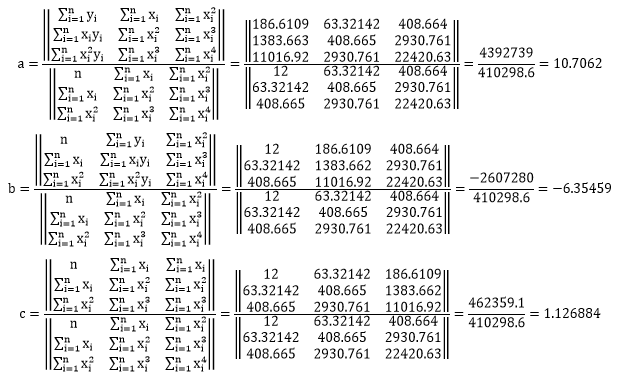
Now this is a very simple equation, so we can simply solve it using Cramer’s rule:
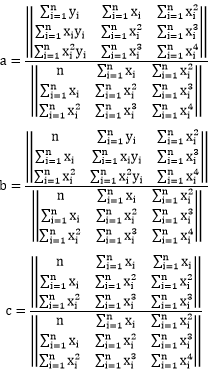
It looks scary but actually not too complex. We need the sum of x, x^2, x^3, x^4, x*y and x^y. We can actually verify this in excel:
| x | y | x^2 | x^3 | x^4 | x*y | x^2*y |
| 9.42 | 52.24 | 88.69578 | 835.323 | 7866.942 | 491.974 | 4633.334 |
| 2.78 | 4.15 | 7.721688 | 21.45697 | 59.62447 | 11.53932 | 32.06537 |
| 5.87 | 13.72 | 34.43254 | 202.0476 | 1185.6 | 80.52797 | 472.5321 |
| 5.49 | 7.00 | 30.18894 | 165.8715 | 911.3719 | 38.47401 | 211.3934 |
| 6.48 | 5.28 | 41.99053 | 272.099 | 1763.204 | 34.19838 | 221.6059 |
| 4.91 | 6.98 | 24.08858 | 118.227 | 580.2595 | 34.23907 | 168.0457 |
| 7.82 | 42.00 | 61.22442 | 479.0568 | 3748.43 | 328.6334 | 2571.426 |
| 2.70 | 7.15 | 7.269068 | 19.59829 | 52.83935 | 19.27266 | 51.96143 |
| 2.65 | 3.41 | 7.003793 | 18.53532 | 49.05312 | 9.028243 | 23.89296 |
| 8.42 | 31.00 | 70.90802 | 597.0945 | 5027.948 | 261.0414 | 2198.149 |
| 5.85 | 12.59 | 34.27254 | 200.6409 | 1174.607 | 73.71933 | 431.5732 |
| 0.93 | 1.09 | 0.869064 | 0.810173 | 0.755272 | 1.014426 | 0.945685 |
| 63.32 | 186.61 | 408.665 | 2930.761 | 22420.63 | 1383.662 | 11016.92 |
So we have:
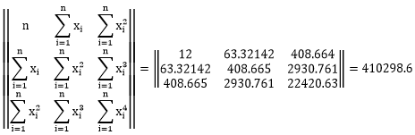
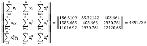

So in the end we get:
This is exactly what Excel displayed on the chart:
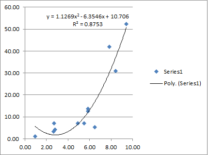
I actually put all this in an Excel file so you can try it yourself. Please note that in the excel file we have a data set of 12 points. If your data set has a different size, you may have to adapt the formulas a little bit. 🙂